This post documents the full aerodynamic design and analysis process for a flying wing UAV, from the initial geometry decisions through meshing, CFD simulation in ANSYS Fluent, grid independence verification, and final wind tunnel validation. The aim was to characterise the wing's performance across its full operating altitude range — from sea level up to 14,000 m — and use those results to drive real design decisions on stall limits, range, and autopilot configuration.
Configuration Selection: Why a Flying Wing
The first design decision was the overall configuration. A conventional tailed aircraft is forgiving to design — the horizontal stabiliser provides a strong pitch-restoring moment that makes stability relatively easy to achieve. A flying wing offers no such safety net: every surface must earn its place, and stability has to be designed into the aerofoil and planform geometry itself.
The tradeoff is efficiency. By eliminating a separate fuselage and tail, a flying wing eliminates surfaces that generate drag without generating lift. The result is a higher lift-to-drag ratio for a given wing area, which directly translates into longer range. For an aircraft that needs to cover tens of kilometres under its own power, that efficiency advantage is decisive.
The Martin Hepperle MH-60 aerofoil was chosen for the section profile. The MH series was developed specifically for tailless aircraft: it produces low torsional moments (critical for pitch stability without a tail), high lift coefficients relative to drag, and is widely used in high-performance sailplanes and flying wings.
Geometry and Aerofoil Selection
The wing geometry was modelled in SolidWorks 2016. The key dimensions are summarised below.
| Parameter | Value |
|---|---|
| Wing span | 2.0 m |
| Root chord | 0.476 m |
| Tip chord | 0.18 m |
| Aspect ratio | 6.324 |
| Aerofoil | MH-60 (tapered to scaled MH-60 at tip) |
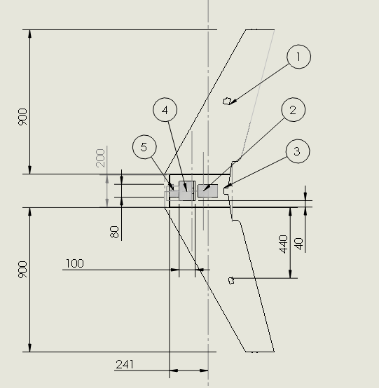
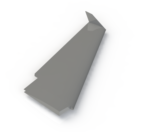
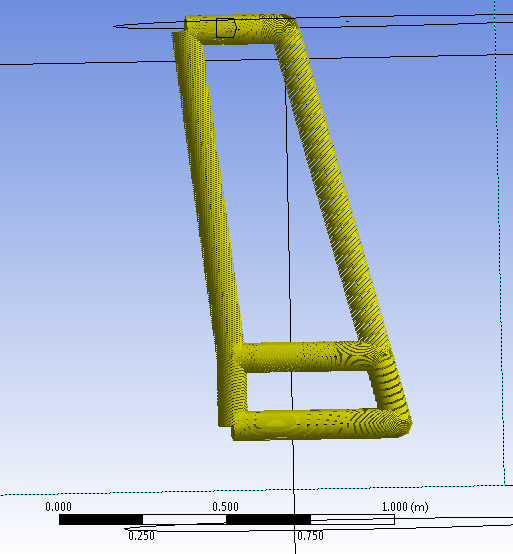
Because the left and right wings are aerodynamically symmetric, only a half-wing model was analysed. Flow over the elevons, winglets, and other small surface features was neglected to keep the mesh tractable. The geometry was exported as IGES and imported into ANSYS Workbench 15.0.
Flow Domain Setup
The flow domain defines the control volume within which Fluent solves the governing equations. Its size and shape must be chosen carefully: too small and the far-field boundaries interfere with the solution; too large and the mesh becomes unnecessarily expensive.
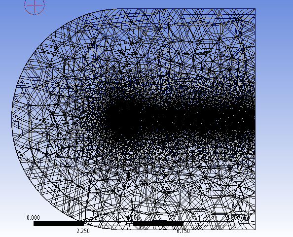
A C-shaped domain was chosen. The C-type grid has two useful properties for external aerodynamics: it naturally captures the wake region behind the trailing edge (important for drag), and it avoids placing many mesh nodes at the corners of a rectangular domain where they would contribute nothing to accuracy.
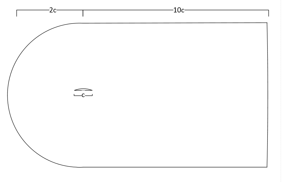
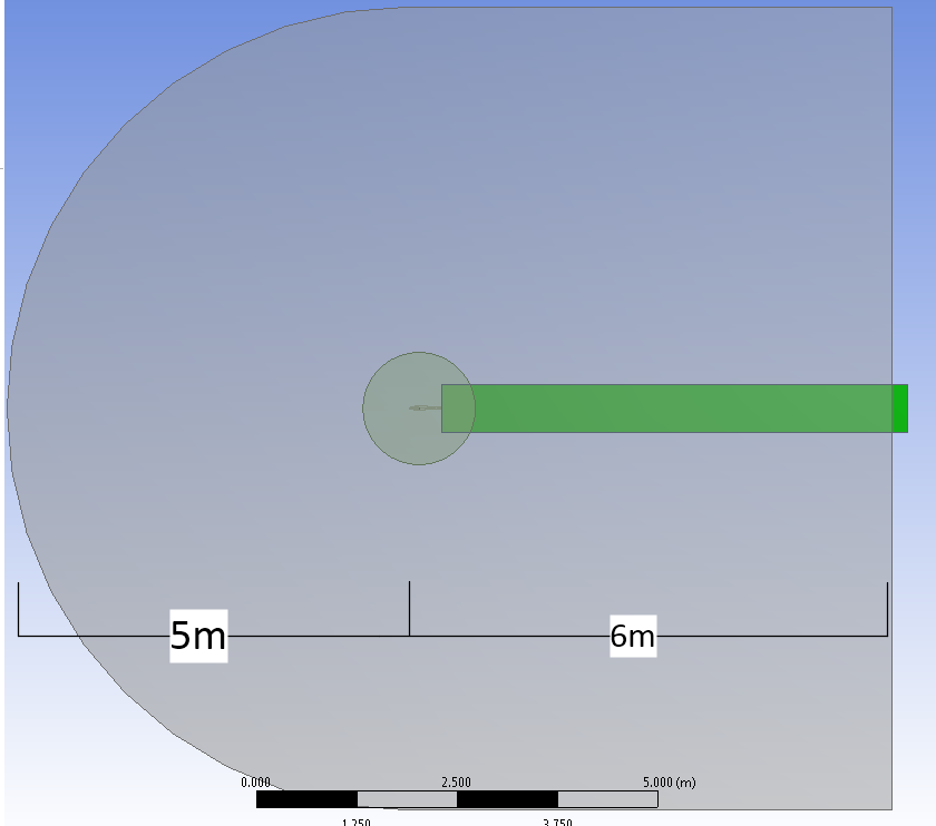
Two additional solid bodies were created inside the main domain: a cylinder closely surrounding the wing and a cuboid in the wake region. These were used as "bodies of influence" to locally refine the mesh without applying that fine sizing everywhere. A Boolean subtraction was used to cut the wing geometry out of the domain, leaving a void representing the solid surface.
The angle of incidence was parameterised in ANSYS, allowing the inclination angle to be swept across the full range of interest without rebuilding the geometry each time.
Meshing Strategy
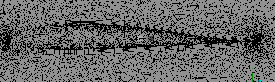
Meshing an external aerodynamics problem requires balancing several competing requirements. The far-field needs to be coarse to keep the element count manageable. The wake needs moderate density to capture the shear layer and turbulent structures. The wing surface and especially the leading and trailing edges need very fine elements to resolve the steep pressure gradients. And the boundary layer on the wing surface needs a structured inflation layer to capture the velocity profile that drives skin friction drag.
Global settings
The physics preference was set to CFD with the advanced sizing function set to curvature. The relevance centre was set to Fine with smoothing set to High. Global minimum element size was 0.0022 m and maximum 0.9 m. The bodies of influence reduced the element size to 0.08 m in the cylindrical and wake refinement zones.
Edge sizing on the wing
Large pressure gradients exist at the leading and trailing edges where flow separates or accelerates sharply. An edge sizing was applied to the wing perimeter using 500 divisions with soft behaviour, concentrating nodes where they are most needed.
Boundary layer inflation
Accurate drag prediction requires resolving the velocity gradient through the boundary layer — the thin region of viscous flow immediately adjacent to the wing surface. An inflation layer was applied to both the upper and lower wing faces using total thickness mode: 5 layers at a growth rate of 1.2, to a total thickness of 0.01 m.
Final mesh
Mesh quality
Three quality metrics were checked: orthogonal quality (target: close to 1), skewness (target: close to 0), and element quality (target: close to 1). All three are plotted below as histograms.
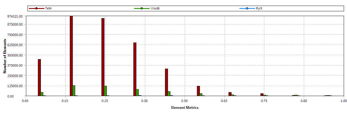
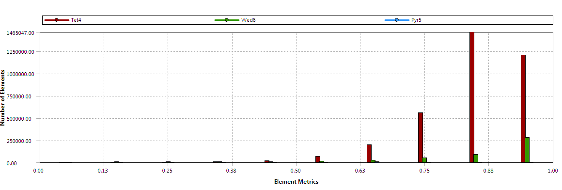
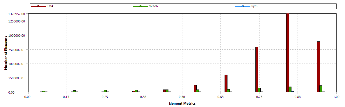
The 3.98 million element mesh was deemed of sufficient quality to proceed. A small number of elements fell into the "acceptable" category (not "good"), but these were located in regions of lower aerodynamic importance away from the wing surface.
Solver Settings and Boundary Conditions
Physical assumptions
The flow at the operating speeds of interest has a Mach number of approximately 0.04, well below the compressibility threshold. The flow was therefore treated as steady-state, viscous, and incompressible. Under these assumptions the continuity and momentum equations simplify, and the energy equation was solved separately to track thermal effects.
Turbulence model: Spalart-Allmaras
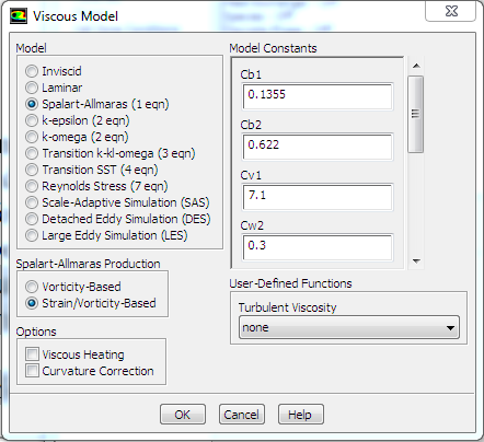
The Spalart-Allmaras (SA) one-equation model was selected from the available RANS approaches. For attached and mildly separated flows at the Reynolds numbers encountered here (Re = 300,000 at sea level; Re = 73,000 at 14,000 m), SA provides a practical balance between accuracy and computational cost. It solves a single transport equation for the modified turbulent kinematic viscosity, making it significantly cheaper than two-equation models such as k-ε or k-ω SST. The rotation and strain production term was selected over the default vorticity-based term for improved accuracy in the deformation tensor calculation.
Boundary conditions
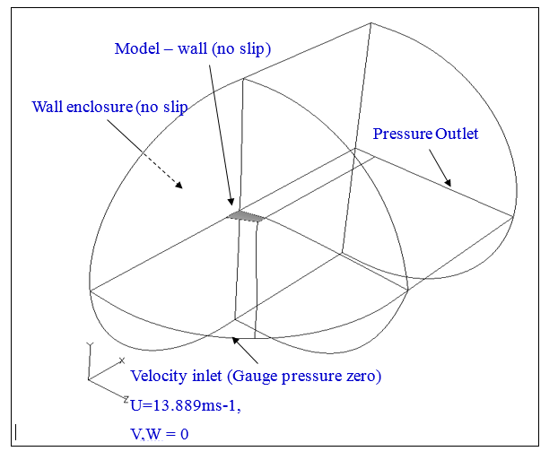
The curved inlet face was defined as a velocity inlet with the velocity vector aligned in the x-direction (parallel to the free stream). A turbulent-to-viscosity ratio of 10 was specified at both inlet and outlet to provide a realistic ambient turbulence level. The outlet was a pressure outlet at zero gauge pressure. The wing surface was a no-slip wall. Air density was set as a parameter, allowing the solver to be re-run at two altitudes by changing a single value: 1.225 kg/m³ at sea level (Re = 300,000) and 0.288 kg/m³ at 14,000 m (Re = 73,000).
Solution scheme
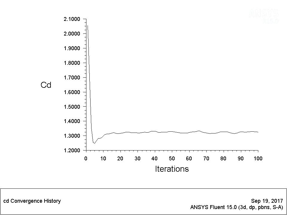
The pressure-based coupled solver was used — recommended for low-speed incompressible flows. Second-order upwind spatial discretisation was applied to momentum and energy for improved accuracy over first-order. Force monitors were configured to track lift and drag components in the x and y directions throughout the iteration. Solutions were run for 130 iterations from a hybrid initialisation; all residuals converged past approximately 40 iterations.
CFD Results
Aerodynamic Efficiency (L/D) vs. Angle of Attack
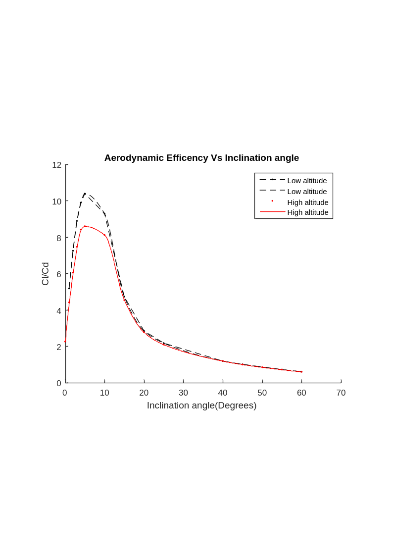
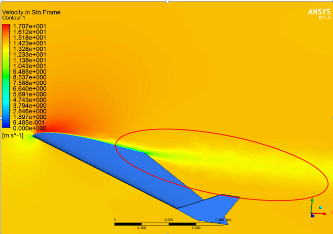
The lift-to-drag ratio peaks at 5° angle of attack for both altitudes: 10.39 at sea level and 8.596 at 14,000 m. Beyond 5°, drag rises rapidly as the turbulent wake behind the trailing edge grows, pulling the efficiency down steeply. The gradual decline from 5° to 10° — rather than an abrupt cliff — is aerodynamically desirable: it gives the pilot or autopilot early warning of an approaching stall rather than a sudden loss of control. The stall angle is therefore defined as 5°, with the onset of full stall occurring at 10°.
Lift and Lift Coefficient vs. Angle of Attack
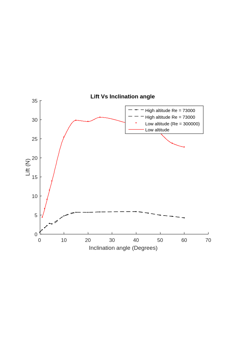
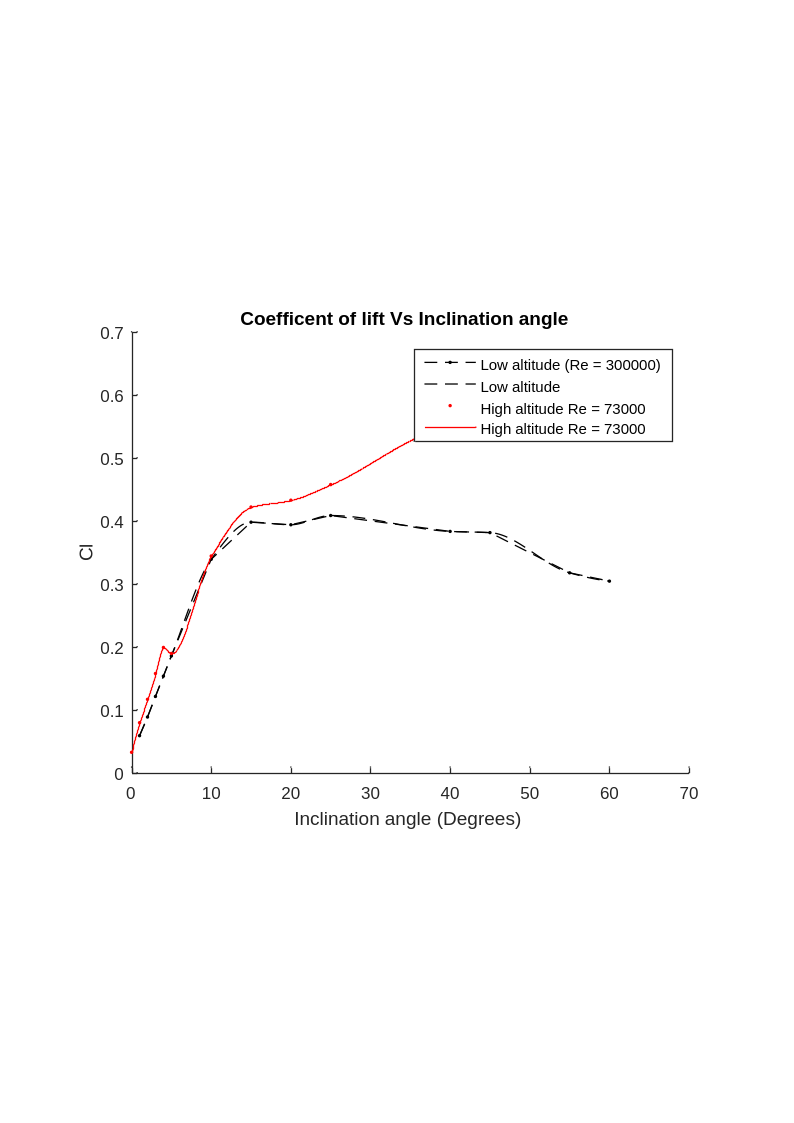
At sea level the half-wing produces 14 N at the stall angle (28 N for the full wing). At 14,000 m this drops to approximately 2.5 N at the critical angle — a dramatic reduction driven entirely by the density difference. The lift coefficient plot reveals something important: Cl itself is nearly unchanged between altitudes. Since lift scales with ρV², an operator can recover lost lift by flying faster. This finding directly informed the cruise speed selection.
Drag and Drag Coefficient vs. Angle of Attack
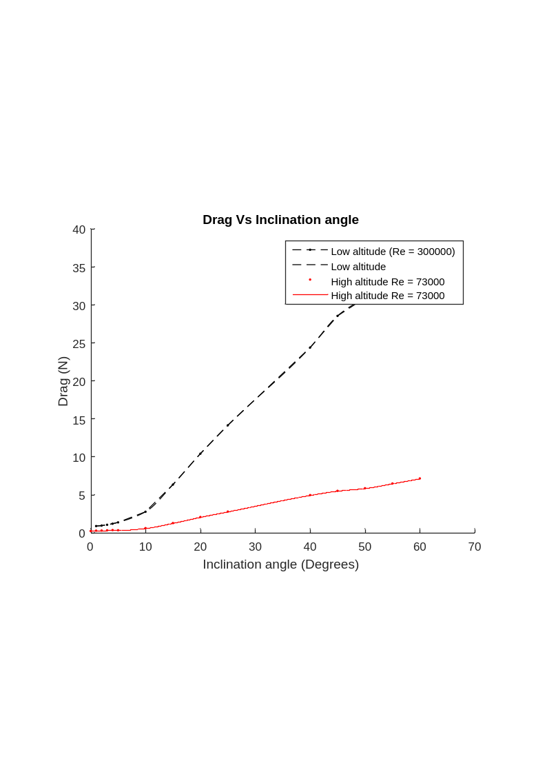
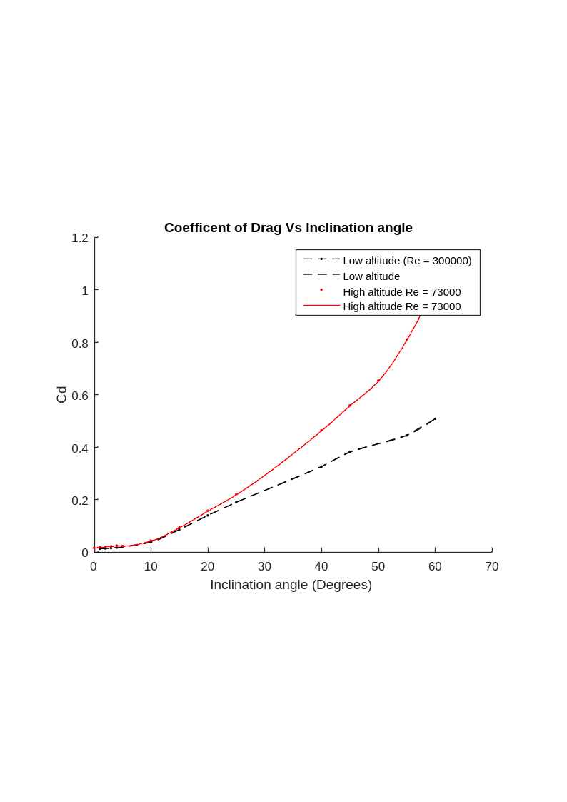
Pitching Moment Coefficient and Longitudinal Stability
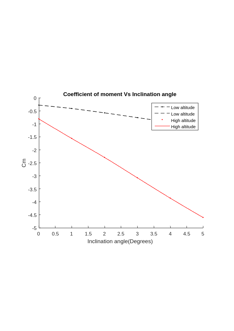
Static longitudinal stability requires that the derivative of the pitching moment coefficient with respect to angle of attack is negative: dCm/dα < 0. If the wing pitches nose-up, the restoring moment must push it back down. Inspecting the Cm vs. AOA plot, the slope is negative at both altitudes throughout the pre-stall range. The flying wing is therefore statically stable in pitch — a non-trivial result for a tailless design, and one that justifies the choice of the MH-60 section, which was specifically engineered for this characteristic.
Stall Speed Derivation
Stall speed is the minimum airspeed at which the wing can generate sufficient lift to support the aircraft weight. It occurs when Cl is maximised (at the stall angle). From the force balance at level flight:
Substituting values (aircraft mass 1.804 kg, wing area 0.56 m², Cl,max from CFD):
| Altitude | ρ (kg/m³) | Cl,max | Vstall |
|---|---|---|---|
| Sea level | 1.225 | 10.39 | 2.23 m/s (8.0 km/h) |
| 14,000 m | 0.228 | 8.596 | 5.58 m/s (20.1 km/h) |
The higher stall speed at altitude was used as the conservative limit programmed into the onscreen display — ensuring the stall warning triggers safely even at low altitude where the margin is greater.
Grid Independence Study
A CFD result is only meaningful if it is independent of the mesh that produced it. The grid independence study tests this by halving the mesh size (body sizing reduced from 0.04 m to 0.02 m) and comparing the results. If the solution changes significantly, the original mesh was too coarse. If it changes negligibly, the solution is considered mesh-converged.
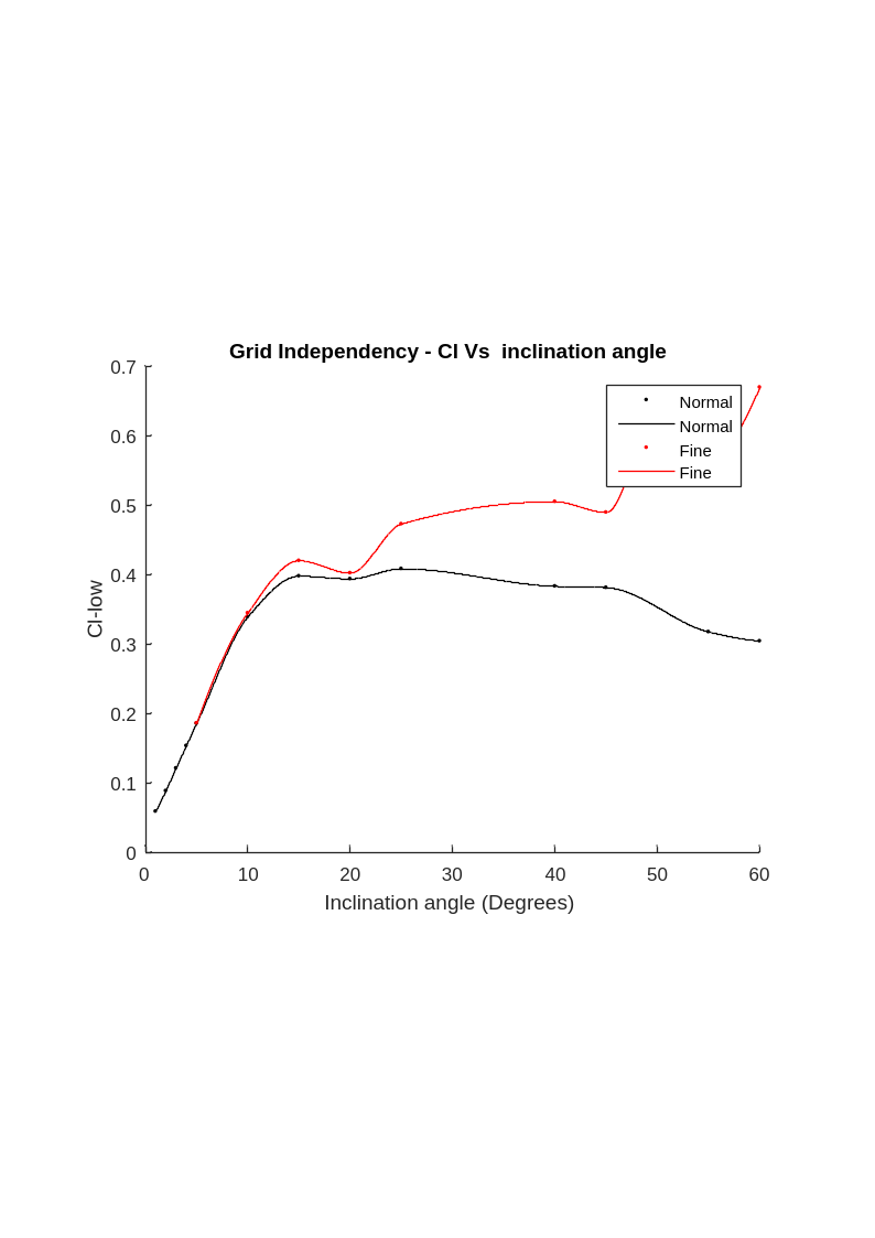
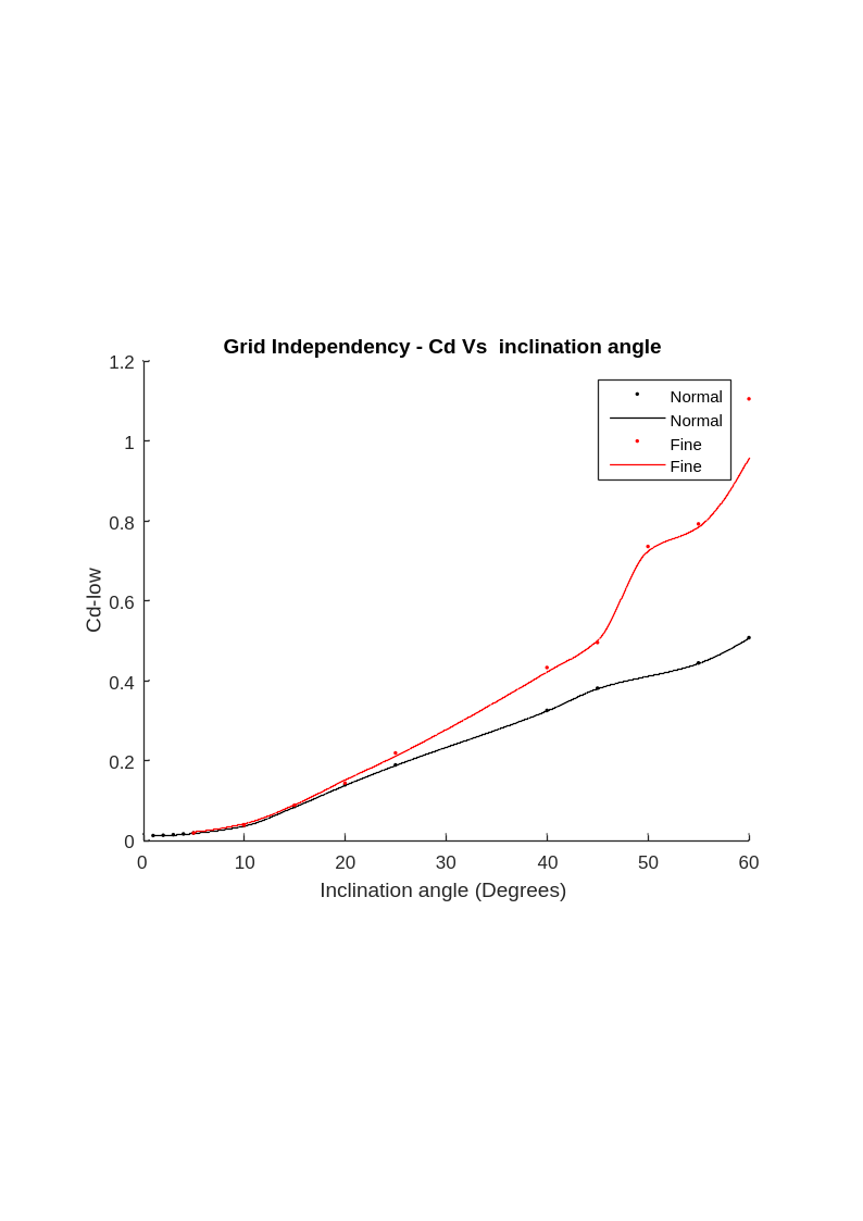
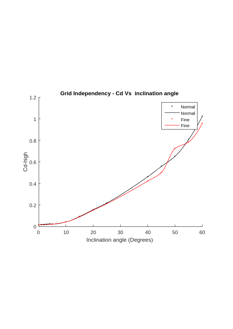
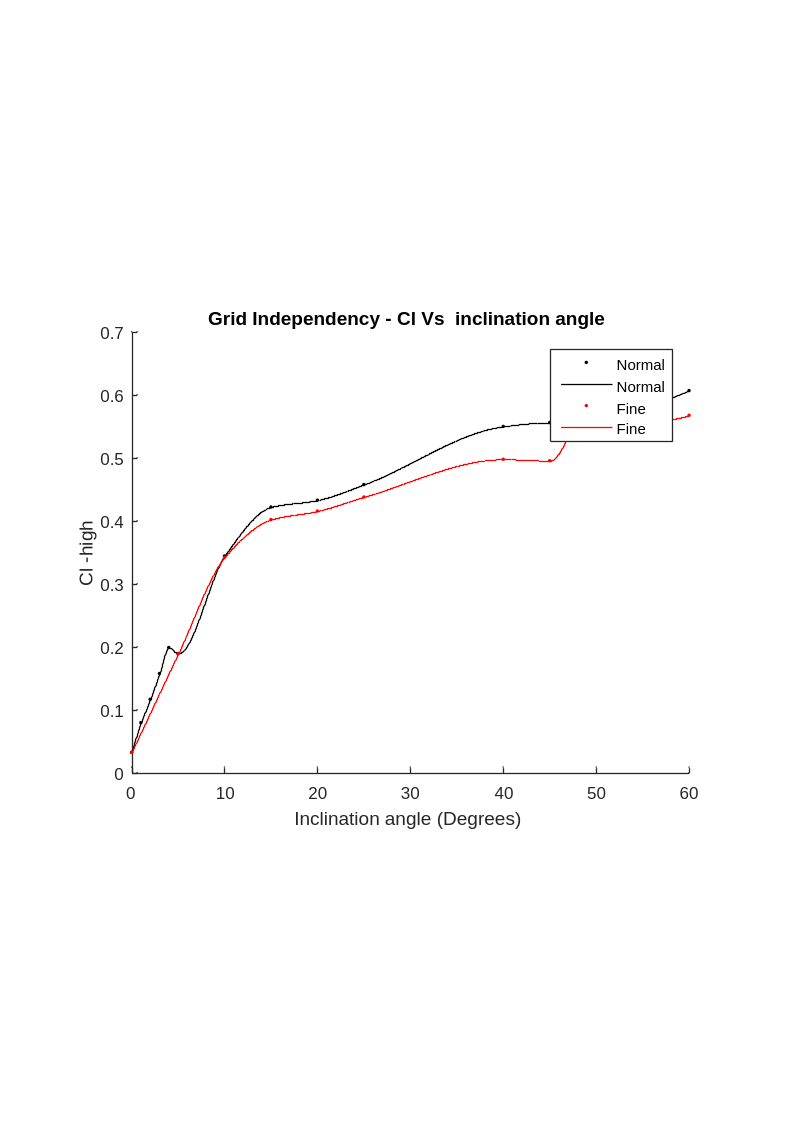
The study confirms that the 3.98 million element mesh is grid-converged in the operating range of interest (0°–10° AOA). Values vary by less than 0.01% before the stall angle. Post-stall divergence is expected: the Spalart-Allmaras model is not designed for massively separated flows, and the mesh topology at those angles is no longer appropriate regardless of refinement. Since the design operates below stall, this limitation is acceptable.
Range Calculation and Motor Bench Test
With the aerodynamic coefficients established, the theoretical range could be calculated from the battery capacity and the thrust required to maintain cruise speed. At level flight the lift equals weight, so:
The thrust required at cruise is determined by the aerodynamic efficiency at that operating point (L/D = 2.253 at cruise Cl = 0.064): T = W / (L/D) = 7.85 N = 0.801 kg of thrust.
To map thrust to current draw, a motor bench test was conducted. The motor and propeller were mounted on a bracket over a weighing scale, and throttle was incremented while recording both thrust and current through a shunt resistor.
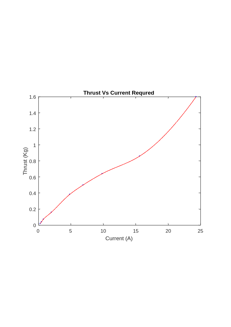
With five 1,500 mAh batteries (7,500 mAh total) and a cruise current draw of 14.28 A, the flight time is 525 seconds. Multiplying by the cruise speed gives a theoretical range of 53.6 km.
Wind Tunnel Validation
Validation is the step that connects CFD results to physical reality. A quarter-scale model of the wing was designed in SolidWorks and 3D-printed in PLA. A load cell was integrated into the model to measure the perpendicular force (lift), and a pitot tube with differential pressure sensor was installed in the tunnel to measure airspeed.
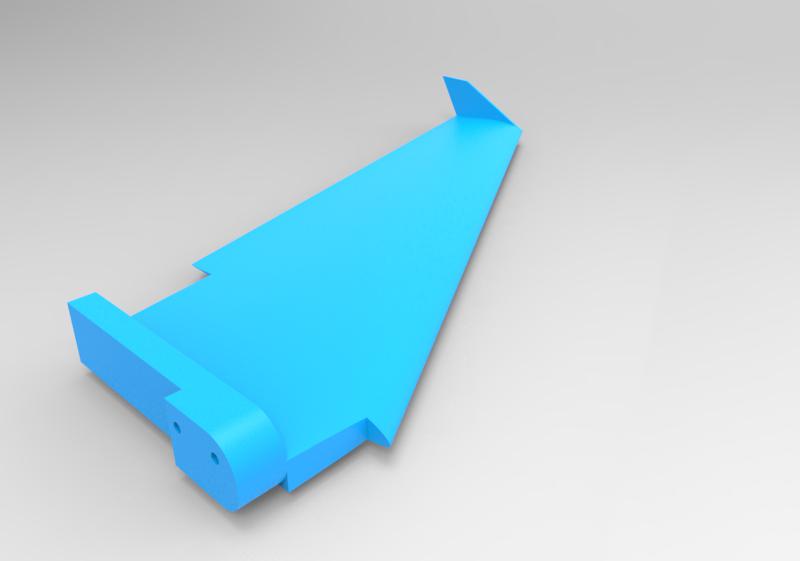
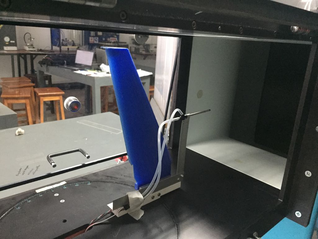
To match Reynolds number between the scale model and the full-size CFD model, the tunnel velocity was increased to compensate for the shorter chord. From Re = ρVl/μ = 300,000, with the mean chord of the quarter-scale model at 0.082 m, the required tunnel speed was 55.4 m/s.
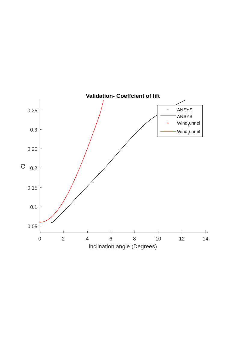
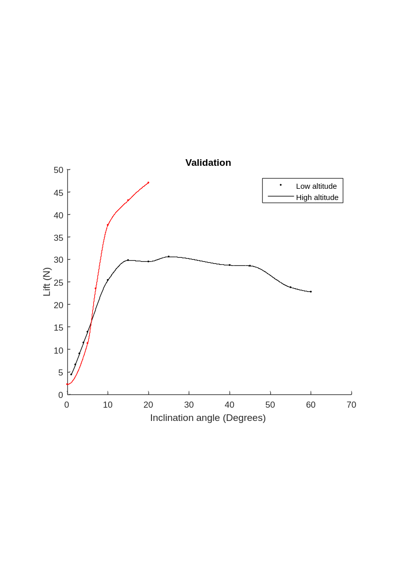
The root mean square error between the CFD and wind tunnel lift coefficients was RMSE = 0.327. While this appears large in absolute terms, the largest discrepancies occur at high AOA readings that are outside the valid operating range of the mesh (and where experimental noise from panel vibration and the leaky tunnel window were significant). Within the 0°–7° pre-stall range, agreement is close and the curve shapes match well. The CFD model was judged sufficiently accurate for its intended purpose.
Fabrication and Test Flight
The prototype was built from extruded polystyrene foam (XPS), chosen for its high rigidity-to-density ratio and low thermal conductivity. Aerofoil templates from SolidWorks were printed at scale and used to guide a home-built hot-wire cutter — a nichrome wire stretched between two posts, heated by a bench power supply — to carve the foam into the correct section profile. Tapered wings require the wire to travel at two different speeds simultaneously (one for root, one for tip), which required several iterations to achieve cleanly.
Three carbon fibre spars were installed to resist aeroelastic flutter: two oriented to resist bending and one offset to resist twist. The electronics bay was reinforced with balsa wood. Servo leads were wrapped in grounded aluminium foil to prevent electromagnetic interference with the control link.
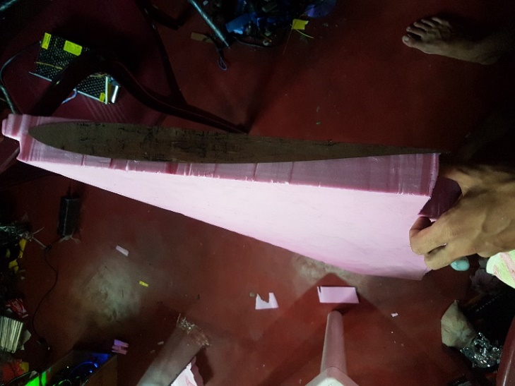
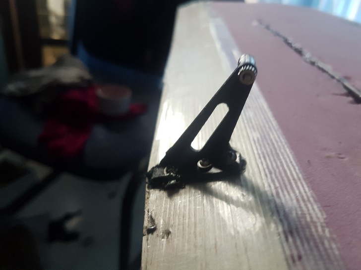
The prototype flew successfully across multiple test sessions. The aerodynamic stability predicted by CFD was confirmed in flight: the aircraft maintained controlled, stable flight without unusual tendencies. The stall speed limits from CFD were programmed into the OSD and respected the behaviour observed in the air. The one identified shortcoming was undersized elevon surfaces, which produced a larger-than-ideal turning radius — a straightforward fix for future iterations.